From Coursera, State Estimation and Localization for Self-Driving Cars by University of Toronto
https://www.coursera.org/learn/state-estimation-localization-self-driving-cars
Least Squares
Ordinary and weighted least squares
Ordinary least squares
example from estimating resistance:
- let the measurement model be: $$y_i = x + v_i$$
- $x$ is the actual resistance
- $v_i$ is the measurement noise
- then the squared error is : $e^2_i = (y_i-x)^2$
- The squared error criterion: $$ \hat x_{LS}=argmin_x (e^2_1+e^2_2+e^2_3+e^2_4) = L_{LS}(x)$$
- the ‘best’ estimate of resistance is the one that minimizes the sum of squared errors.
- rewrite into vector form: $$ e= y- H x$$
- $H$ is called Jacobian: $[1 1 1 1]^T$
- therefore, $$L_{LS}(x) = (e^2_1+e^2_2+e^2_3+e^2_4) = e^Te$$ $$=(y-Hx)^T(y-Hx)$$ $$=y^Ty - x^TH^Ty - y^THx + x^TH^THx$$
- therefore, the rest thing is to minimize the above equation
- get partial derivative with respect to the parameter, set to 0:
$$\frac{\partial L}{\partial x}|_{x=\hat x} = -y^TH-y^TH+2\hat x^T H^TH=0$$ $$-2y^TH+2\hat x^TH^TH=0$$ - re-arrange, we get (when H is full-column rank) $$\hat x_{LS} = (H^TH)^{-1} H^Ty$$
- Assumptions:
- Our measurement model,$y=x+v$,is linear
- Measurements are equally weighted (we do not suspect that some have more noise than others)
weighted least squares
The same example: Suppose we take measurements with multiple multimeters,some of which are better than others
- Consider the general linear measurement model for m measurements and n unknowns: $$y = Hx+v$$
- In regular least squares, we implicitly assumed that each noise term was of equal variance: $$E(v^2_i) = \sigma^2 (i=1,…,m)$$ $$R=E(vv^T) = diag(\sigma^2,…,\sigma^2)$$
- If we assume each noise term is independent, but of different variance
$E(v^2_i) = \sigma_i^2 (i=1,…,m)$, $R=E(vv^T) = diag(\sigma_1^2,…,\sigma_m^2)$ - Then we can define a weighted least squares criterion as: $$L_{WLS}(x)=e^TR^{-1}e = \frac{e^2_1}{\sigma^2_1} + \frac{e^2_2}{\sigma^2_2} + … + \frac{e^2_m}{\sigma^2_m}$$, where $e = y-Hx$
- expanding the new criterion: $$L_{WLS}(x) = e^TR^{-1}e = (y-Hx)^TR^{-1}(y-Hx)$$
- get the derivative: $$\frac{\partial L}{\partial x}|_{x=\hat x} = 0 = -y^TR^{-1}H + \hat x^T H^TR^{-1}H$$
- get $$H^T R^{-1} H \hat x_{WLS} = H^TR^{-1}y$$
- the weighted normal equation: $$\hat x = (H^TR^{-1}H)^{-1} H^T R^{-1}y$$
Comparison between ordinary and weighted least squares: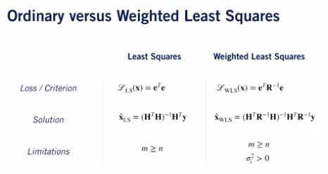
Summary:
- Measurements can come from sensors that have different noisy characteristics
- Weighted least squares lets us weight each measurement according to noise variance
Recursive least squares
In the above example, what if we have a stream of data?
We can use linear recursive estimator
- Suppose we have an optimal estimate, $\hat X_{k-1}$, of our unknown parameters at time k-1
- Then we obtain a new measurement at time k: $y_k = H_kx+v_k$
- We can use a linear recursive update: $\hat x_k = \hat x_{k-1} + K_k(y_k-H_k \hat x_{k-1})$
- We update our new state as a linear combination of the previous best guess and the current measurement residual (or error), weighted by a gain matrix $K_k$
- What is teh gain matrix?
- We can compute the gain matrix by minimizing a similar least squares criterion, but this time we’ll use a probabilistic formulation
- We wish to minimize the expected value of the sum of squared errors of our current estimate at time step k: $$L_{RLS} = E[(x_k-\hat x_k)^2]=\sigma_k^2$$
- If we have n unknown parameters at time step k,we generalize this to $$L_{RLS} = E[(x_{1k}-\hat x_{1k})^2 + … +(x_{nk}-\hat x_{nk})^2] = Trace(P_k)$$
- $P_k$ is the estimator covariance
- Using linear recursive formulation, we can express covariance as a function of $K_k$: $$P_k = (1-K_kH_k)P_{k-1} (1-K_kH_k)^T + K_kR_kK^T_k$$
- We can show(through matrix calculus) that this is minimized when $$K_k = P_{k-1}H^T_k(H_kP_{k-1}H^T_k + R_k)^{-1}$$
- With this expression, we can also simplify our expression for $P_k$: $$P_k = P_{k-1} - K_kH_kP_{k-1} = (1-K_kH_k)P_{k-1}$$
Recursive Least Squares I Algorithm
- Initialize the esimator: $$\hat x_0 = E[x]$$ $$P_0 = E[(x-\hat x_0)(x-\hat x_0)^T]$$
- Set up the measurement model,defining the Jacobian and the measurement covariance matrix: $$y_k = H_kx+v_k$$
- Update the estimate of $\hat x_k$ and the covariance $P_k$ using: $$K_k = P_{k-1}H^T_k(H_kP_{k-1}H^T_k +R_k)^{-1}$$ $$\hat x_k = \hat x_{k-1} + K_k(y_k-H_k\hat x_{k-1}) $$ $$P_k = (1-K_kH_k)P_{k-1}$$
Summary
- RLS produces a ‘running estimate’ of parameter(s)for a stream of measurements
- RLS is a linear recursive estimator that minimizes the (co)variance of the parameter(s) at the current time
Maximum likelihood and the method of least squares
The maximum likelihood estimate, given additive Gaussian noise, is equivalent to the least squares or weighted least squares solutions we derived earlier.
Summary:
- LS and WLS produce the same estimates as maximum likelihood assuming Gaussian noise
- Central Limit Theorem states that complex errors will tend towards a Gaussian distribution
- Least squares estimates are significantly affected by outliers