From Coursera, State Estimation and Localization for Self-Driving Cars by University of Toronto
https://www.coursera.org/learn/state-estimation-localization-self-driving-cars
LIDAR Sensing
Light Detection and Ranging Sensors
The operating principles of LIDAR sensors
- For a basic LIDAR in one dimension, it has three components: a laser, a photodetector, and a very precise stopwatch.
- The laser first emits a short pulse of light usually in the near infrared frequency band along some known ray direction. At the same time, the stopwatch begins counting. The laser pulse travels outwards from the sensor at the speed of light and hits a distant target.
- As long as the surface of the target isn’t too polished or shiny, the laser pulse will scatter off the surface in all directions, and some of that reflected light will travel back along the original ray direction. The photodetector catches that return pulse and the stopwatch tells you how much time has passed between when the pulse first went out and when it came back. That time is called the round-trip time.
- then the distance from the LIDAR to the target is simply half of the round-trip distance calculated by the time and the speed of the light
- This technique is called time-of-flight ranging
- the photodetector also tells the intensity of the return pulse relative to the intensity of the pulse that was emitted. This intensity information is less commonly used for self-driving, but it provides some extra information about the geometry of the environment and the material the beam is reflecting off of.
The basic LIDAR sensor models in 2D and 3D
- But how do to use the above knowledge to measure a whole bunch of distances in 2D or in 3D?
- The trick is to build a rotating mirror into the LIDAR that directs the emitted pulses along different directions.
- As the mirror rotates, you can measure distances at points in a 2D slice around the sensor.
- If you then add an up and down nodding motion to the mirror along with the rotation, you can use the same principle to create a scan in 3D.
- Measurement Models for 3D LIDAR Sensors
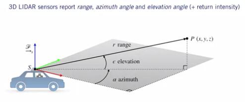
- LIDARs measure the position of points in 3D using spherical coordinates, range or radial distance from the center origin to the 3D point, elevation angle measured up from the sensors XY plane, and azimuth angle, measured counterclockwise from the sensors x-axis.
- The azimuth and elevation angles are measured using encoders that tell you the orientation of the mirror, and the range is measured using the time of flight as we’ve seen before.
- suppose we want to determine the cartesian XYZ coordinates of our scanned point in the sensor frame, which is something we often want to do when we’re combining multiple LIDAR scans into a map. To convert from spherical to Cartesian coordinates, we use the inverse sensor model: $$[x \; y \; z]^T = h^{-1}(r,\alpha, \varepsilon) = [r\cos\alpha \cos \varepsilon \quad r \sin \alpha \cos \varepsilon \quad r \sin \varepsilon]^T$$ where $\alpha$ is the azimuth angle, $\varepsilon$ is the elevation angle
- Therefore, the forward sensor model is: (which from Cartesian coordinates to spherical coordinates) $$[r \alpha \varepsilon]^T = h(x,y,z) = [\sqrt{x^2+y^2+z^2} \tan^{-1}(\frac yx) \sin^{-1}(\frac{z}{\sqrt{x^2+y^2+z^2}})]^T$$
The major sources of measurement error for LIDAR sensors
- Uncertainty in determining the exact time of arrival of the refected signal
- Uncertainty in measuring the exact orientation of the mirror
- Interaction with the target(surface absorption, specular reflection, etc.): e.g.: if the surface is completely black, it might absorb most of the laser pulse. Or if it’s very shiny like a mirror, the laser pulse might be scattered completely away from the original pulse direction.
- Variation of propagation speed (e.g., through materials)
- These factors are commonly accounted for by assuming additive zero-mean Gaussian noise on the spherical coordinates with an empirically determined or manually tuned covariance.
- Motion Distortion
- Typical scan rate for a 3D LIDAR is 5-20 Hz
- For a moving vehicle, each point in a scan is taken from a slightly different place
- Need to account for this if the vehicle is moving quickly, otherwise motion distortion becomes a problem
LIDAR Sensor Models and Point Clouds
The basic point cloud data structure
- assign an index to each of the points, say point 1 through point n, and store the x, y, z coordinates of each point as a 3 by 1 column vector
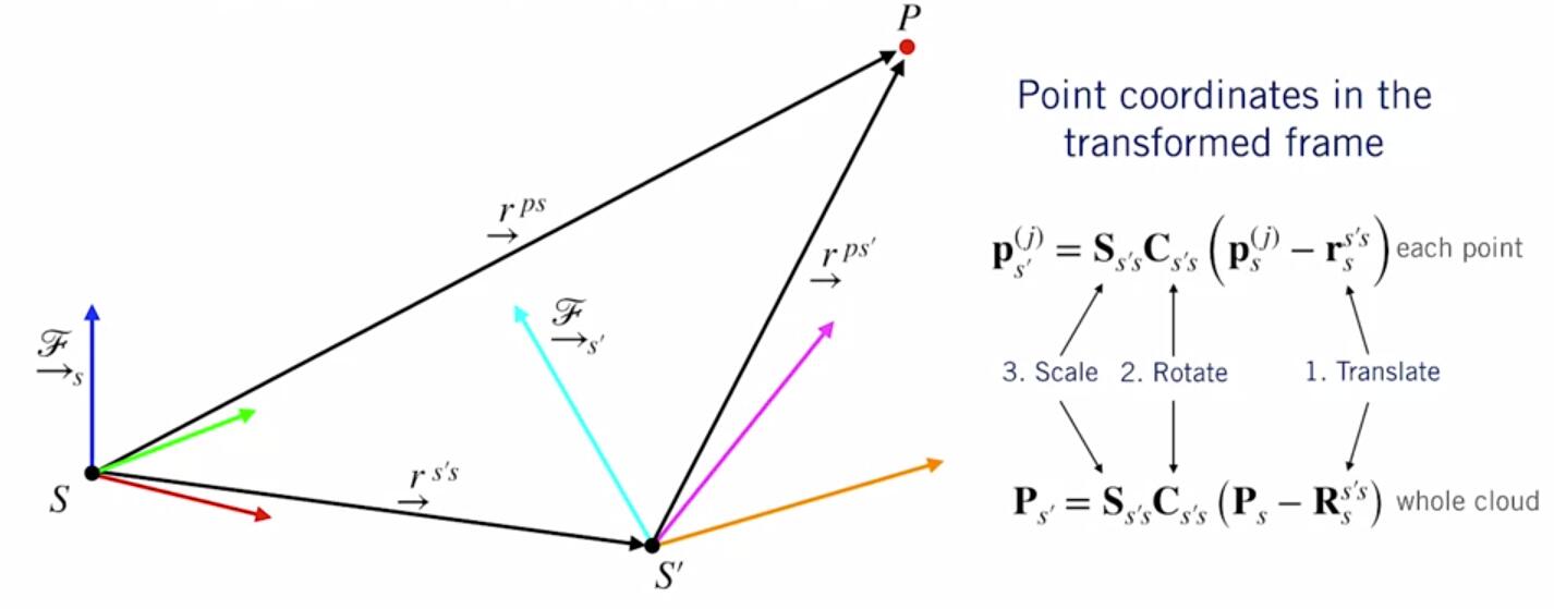
Common spatial operations on point clouds
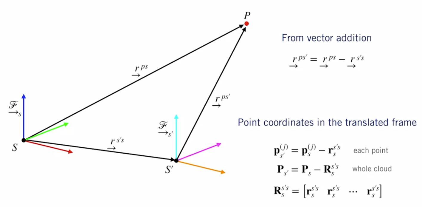
- Translation
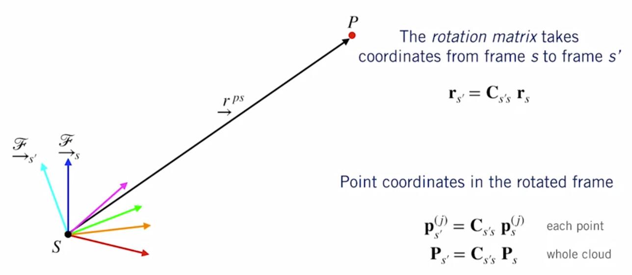
- Rotation
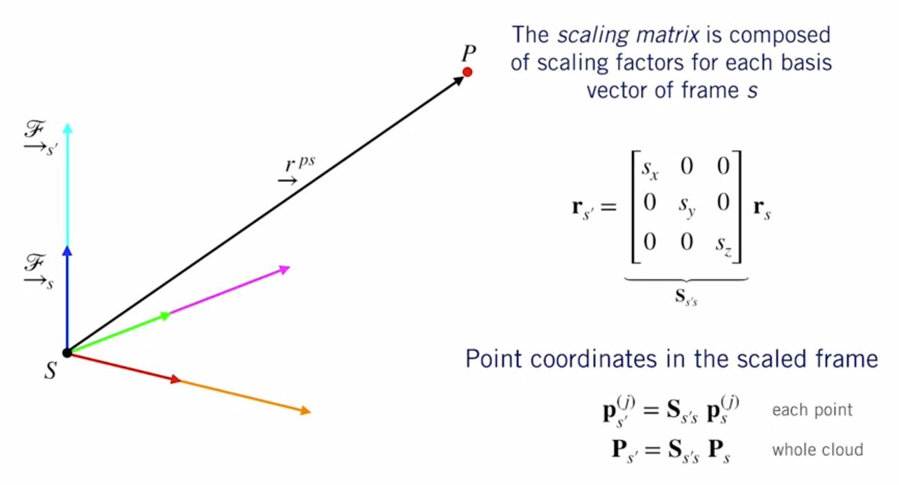
- Scaling
- Put them together
Least squares to fit a plane to a point cloud
- Plane fitting
- One of the most common and important applications of plane-fitting for self-driving cars is figuring out where the road surface is and predicting where it’s going to be as the car continues driving.
- we have a bunch of measurements of x, y and z from our LIDAR point cloud, and we want to find values for the plane by the parameters a, b, and c defined: $z=a+bx+cy$
- to find the best fit, we use least-squares estimation
- define a measurement error $e$ for each point in the point cloud: $e_j = \hat z_j - z_j = (\hat a + \hat bx_j + \hat c y_j) - z_j \quad j=1,…n$
- We can stack all of the measurement errors into matrix form, ad minimize the squared-error criterion to get the least-squares solutions for the parameters
- Open-source Point Cloud Library(PCL) has many useful functions for doing basic and advanced operations on point clouds in C++
Pose Estimation from LIDAR Data
Point set registration problem
- one of the most important problems in computer vision and pattern recognition. used to estimate the motion of a self-driving car from point clouds
- the point set registration problems says, given 2 point clouds in two different coordinate frames, and with the knowledge that they correspond to or contain the same object in the world, how shall we align them to determine how the sensor must have moved between the two scans?
- More specifically, we want to figure out the optimal translation and the optimal rotation between the two sensor reference frames that minimizes the distance between the 2 point clouds.
- ICP is the most popular algorithm to solve this problem.
Iterative Closest Point(ICP) algorithm
- Intuition: When the optimal motion is found, corresponding points will be closer to each other than to other points
- Heuristic:For each point,the best candidate for a corresponding point is the point that is closest to it right now
- Steps of ICP:
- Get an initial guess for the transformation ${\check C_{S’S}, \check r^{S’S}_{S}}$:
- the initial guess can come from a number of sources.
- One of the most common sources is a motion model, which could be supplied by an IMU or by wheel odometry or something really simple like a constant velocity or even a zero velocity model
- How complex the motion model needs to be to give us a good initial guess really depends on how smoothly the car is driving.
- If the car is moving slowly relative to the scanning rate of the LIDAR sensor, one may even use the last known pose as the initial guess.
- Associate each point in $P_{S’}$ with the nearest point in $P_S: transform the coordinates of the points in one cloud into the reference frame of the other
- Solve for the optimal transformation ${\hat C_{S’S}, \hat r^{S’S}_S}$
- Repeat until convergence
- Get an initial guess for the transformation ${\check C_{S’S}, \check r^{S’S}_{S}}$:
- Solving for the Optimal Transformation
- use least-squares:
- Special attention need to be paid to the rotation matrix: as two rotation matrices addition will not necessarily results in a valid rotation matrix. 3D rotations belong to something called the special orthogonal group or SO3
- Steps:
- Compute the centroids of each point cloud:
- $\mu_S = \frac 1n \sum^n_{j=1}P^{j}_S$
- $\mu_{S’} = \frac 1n\sum^n_{j=1}P^{(j)}_{S’}$
- Compute a matrix capturing the spread of the two point clouds: $$W_{S’S} = \frac 1n \sum^n_{j=1}(P^{(j)}{s} - \mu_{S})(P^{(j)}{s’}-\mu_{S’})^T$$ this W matrix can be regarded as something like an inertia matrix you might encounter in mechanics.
- finding the optimal rotation matrix using SVD of W matrix: $$USV^T = W_{S’S}$$ where U V are rotation and S is the scaling matrix. As we’re dealing with rigid body motion in this problem, we don’t want any scaling in a rotation estimate, so we’ll replace the S matrix with something like the identity matrix to remove the scaling.
- Use the optimal rotation to get the optimal translation by aligning the centroids
- Compute the centroids of each point cloud:
- Estimate the uncertainty:
- We can obtain an estimate of the covariance matrix of the ICP solution using a formula
- This expression tells us how the covariance of the estimated motion parameters is related to the covariance of the measurements in the two point clouds using certain second-order derivatives of the least squares cost function.
- Variants
- Point-to-point ICP minimizes the Euclidean distance between each point in $P_{S’}$, and the nearest point in $P_S$
- Point-to-plane ICP minimizes the perpendicular distance between each point in $P_{S’}$, and the nearest plane in $P_S$·
- This tends to work well in structured environments like cities or indoors
- first fit a number of planes to the first point cloud and then minimize the distance between each point in the second cloud and its closest plane in the first cloud.
Common pitfalls of the ICP algorithm
- Outliers - Objects in Motion:
- be careful to exclude or mitigate the effects of outlying points that violate our assumptions of a stationary world
- One way to do this is by fusing ICP motion estimates with GPS and INS estimates.
- Another option is to identify and ignore moving objects, which we could do with some of the computer vision techniques.
- But an even simpler approach for dealing with outliers like these is to choose a different loss function that is less sensitive to large errors induced by outliers than our standard squared error loss, Robust Loss Functions: