From Coursera, State Estimation and Localization for Self-Driving Cars by University of Toronto
https://www.coursera.org/learn/state-estimation-localization-self-driving-cars
An Autonomous Vehicle State Estimator
State Estimation in Practice
Accuracy Requirements
- How accurate does the estimator need to be for safe self-driving?
- Typically less than a meter for highway lane keeping
- Less for driving in dense trafic
- GPS accuracy is 1-5 meters in optimal conditions
- Need additional sensors!
Speed Requirements
- How fast do we need to update the vehicle state to ensure safe driving?
- How much computation power does the vehicle have on-board?
- How much power can our computing resources consume?
Localization Failures
- How can localization fail?
- Sensors fail or provide bad data (e.g., GPS in a tunnel)
- Estimation error (e.g, linearization error in the EKF)
- Large state uncertainty (e.g, relying on IMU for too long)
Multisensor Fusion for State Estimation
Develop an error state extended Kalman Filter for estimating position, velocity and orientation using an IMU, GNSS sensor, and LIDAR.
Why use GNSS with IMU & LIDAR?
- Eror dynamics are completely different and uncorrelated
- IMU provides ‘smoothing’ of GNSS, fill-in during outages due to jamming or maneuvering
- Wheel odometry is also possible (if only 20 position orientation is desired)·
- GNSS provides absolute positioning information to mitigate IMU drift
- LIDAR provides accurate local positioning within known maps
Types of EKF coupling
- Tightly coupling:
- use the raw pseudo range and point cloud measurements from our GNSS and LIDAR as observations
- GNSS/LIDAR Measurement: Pseudo-ranges to satellites LIDAR point clouds
- Accuracy: potentially Higher
- Complexity: Higher
- Loosely
- assume data has already been preprocessed to produce a noisy position estimate
- GNSS/LIDAR Measurement: Position
- Accuracy: potentially lower
- Complexity: Lower
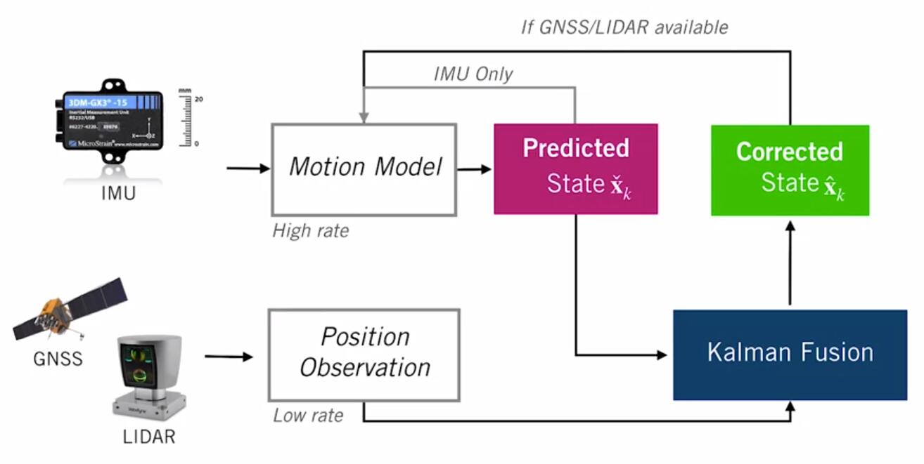
EKF - IMU+GNSS+LIDAR
- use the IMU measurements as noisy inputs to the motion model. This will give us our predicted state, which will update every time we have an IMU measurement. This can happen hundreds of times a second.
- Then we incorporate GNSS and LIDAR measurements whenever they become available(at a much slower rate, say once a second or slower), and use them to correct our predicted state
- What is state?
- we’ll use a 10-dimensional state vector that includes a 3D position, a 3D velocity, and a 4D unit quaternion that will represent the orientation of our vehicle with respect to a navigation frame. $$x_k=[p_k \; v_k \; q_k]^T \in R^{10}$$
- assume that IMU output specific forces and rotational rates in the sensor frame, and combine them into a single input vector u. - note that we’re not going to track accelerometer or gyroscope biases. These are often put into the state vector, estimated, and then subtracted off of the IMU measurements. For clarity, we’ll emit them here and assume our IMU measurements are unbiased.
- therefore, the motion model input will consist of specific force and rotational rates from IMU: $$u_k = [f_k \; \omega_k]^T \in R^6$$
- Loop
- Update state with IMU inputs
- Propagate uncertainty
- If GNSS or LIDAR position available:
- Compute Kalman gain
- Compute error state
- Correct predicted state
- Computed orrected covariance
Sensor Calibration - A Necessary Evil
Intrinsic Calibration
- deals with sensors specific parameters
- ways to get the parameters:
- Manufacturer specifications
- Measure by hand
- Estimate as part of the state
Extrinsic Calibration
- deals with how the sensors are positioned and oriented on the vehicle
Temporal Calibration
- deals with the time offset between different sensor measurements
- ways to deal with
- Assume zero
- Hardware synchronization
- Estimate as part of the state