neural network theory
Interpreting Network Behavior
Extracting and Visualizing Activations:
- use the
activationsfunction to extract features from an input image:- it accepts three inputs: the network, the input image, and the layer to extract features from.
features = activations(net,img,layerName)
- Each convolution layer consists of many 2-D arrays called channels.
- Most CNNs learn to detect features like color and edges in the first convolution layer. In deeper layers, the network learns more complicated features.
- use the function
mat2grayto normalize the activations - use
montageto show the images side by side
Representing Signal Data as Images
- CNN use the images as input, which means every 2-D array can be input to CNN. Therefore, we can represent the signals in to 2-D array for use of CNN
- There are two ways to convert 1-D signal to images: use
spectrogramor a continuous wavelet transform usingcwt.
Feature Extraction for Machine Learning:
- It is difficult to perform deep learning on a computer without a GPU because of the long training time.
- An alternative is to use pretrained networks for feature extraction. Then you can use traditional machine learning methods to classify these features.
- CNNs learn to extract useful features while learning how to classify image data. As you’ve seen, the early layers read an input image and extract features. Then, fully connected layers use these features to classify the image.
- With deep learning, you can use the
activationsfunction to extract features. These features can be used as the predictor variables for machine learning. - We can set the
OutputAsoption to store the features from activation as rows for the machine learning model:testFeatures = activations(net,testImgs,'fc7','OutputAs','rows')
1 | # extract the features from a pretrained net |
Create Networks
Many pretrained networks need the input to be 3-D data and some restriction for the size of the images. If the data you want to train doesn’t satisfy these requirment (like the have more than 3 dimensions), we then need to build our own model.
Create Network Architectures
- The first layer of any convolutional neural network is an image input layer. Function
imageInputLayer(inputSize)can do this. The input size is a three-element vector corresponding to the height, width, and number of channels of that image:inLayer = imageInputLayer([28 28 3]) - Convolution layers learn features in the input image by applying different filters to the image. To create a convolution layer, you need to specify the filter size and the number of filters:
convolution2dLayer([h w],n),convLayer = convolution2dLayer([5 5],20) - Convolution layers are generally followed by rectified linear unit (ReLU) and max pooling layers.
- A ReLU layer sets all negative values to zero:
reluLayer(). The function does not require any inputs. - Max pooling layers perform down-sampling by “pooling” rectangular regions together and computing the maximum of each region. Use the pool size as input:
maxPooling2dLayer([h w]) - The last three layers of a convolutional neural network are
- fullyConnectedLayer: it requires the output size as input. This is the number of classes that the network can predict.
- softmaxLayer: does not require any inputs.
- classificationLayer: does not require any inputs.
- To train a network, we need an array of your entire network architecture. The last step is to stack all the layers you have created into a single array.
1 | # To create an architecture that can be used to classify 28-by-28 color images into two classes. |
Understanding Neural Networks
- Each layer in the network performs some operation on its inputs and outputs a new value.
- The first layer is an image input layer. This layer defines the input size of the network and normalizes the input images. By default, an image input layer subtracts the mean image of the training data set. This centers the images around zero.
- 2-D convolution layers apply sliding filters to the input image. Convolution layers are a key part of the CNN architecture. They rely on the spatial structure of the input image.
- Convolution layers are usually followed by a nonlinear activation layer such as a rectified linear unit (ReLU). A ReLU layer performs a threshold operation to each element of the input. Any value less than zero is set to zero.
- A maximum pooling layer performs down-sampling by dividing the input into rectangular pooling regions and computing the maximum of each region. Pooling reduces the network complexity and creates a more general network.
- Features passing through the network are stored in a collection of matrices until they reach the fully connected layer. At the fully connected layer, the input is “flattened” (which means to tansform the matrix to a vector) so that it can be mapped to the output classes. This layer is a classical neural network.
- The output size for this layer is the number of classes for your classification problem. For example, if you were classifying cats and dogs, the output size would be two.
- The softmax layer converts the values for each output class into normalized scores using a normalized exponential function. You can interpret each value as the probability that the input image belongs to each class.
- The softmax layer converts the values for each output class into normalized scores using a normalized exponential function. You can interpret each value as the probability that the input image belongs to each class.
- The classification output layer returns the name of the most likely class.
Convolutional Layers
- Convolution layers in CNNs perform convolution using learned filters.
- A matrix called a kernel is used to filter the image.
- We can use kernel with the
conv2function to apply a filter to an image:filteredim = conv2(kernel,im) - Using empty brackets as the second input in
imshowwill scale the display based on the minimum and maximum values present in the image:imshow(im,[]) - Or you can also use the
imfilterfunction to apply the same kernels to the entire RGB image, which means the 3-D data.conv2can only apply to a 2-D image.
Summary
List of layer functions
Train Networks
Understand the network training:
- Mini-Batch
- Learning rate
- Learning algorithm
Monitor Training Progress
- can use the
Plotsoption to monitor network training:options = trainingOptions('sgdm','MaxEpochs',2,'InitialLearnRate',0.0001,'Plots','training-progress');
Validation
- About different dataset:
- Training data: used during training to update weights.
- Validation data: used during training to evaluate performance.
- Testing data: used after training to evaluate performance.
- Validation data is useful to detect if your network is overfitting. Even if the training loss is decreasing, if the validation loss is increasing, you should stop training because the network is learning details about the training data that aren’t relevant to new images.
- There are three training options related to validation.
ValidationData: Validation data and labels.ValidationFrequency: Number of iterations between each evaluation of the validation data.ValidationPatience: The number of validations to check before stopping training. Fluctuations in the loss from one iteration to another are normal, so you generally don’t want to stop training as soon as the validation loss increases. Instead, perform several validations. If the loss has not reached a new minimum in that time, then stop the training.
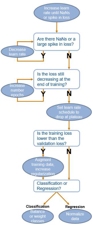
Improve Performance
After testing on the test dataset, if the accuracy is not adequate. We need to improve the network. Any of the inputs to trainNetwork can be modified to train a different network that may perform better.
- From training algorithm options: Modifying the training options is generally the first place to begin improving a network.
- Training Data: If no enough training data, the network may not generalize to new data. If you cannot get more training data, augmentation is a good alternative.
- Architecture: If you are performing transfer learning, you often do not need to modify the network architecture to train an effective network. One alternative is to try using a pretrained network with a directed acyclic architecture like GoogLeNet or ResNet-50.
Training Options:
- Decrease learning rate: If there is a large spike in loss, or loss values are no longer being plotted, your initial learning rate is probably too high. Decrease the learning rate by a power of ten until your loss decreases.
- When you train a network, there is always a trade-off between accuracy and training time.
- The following chart shows some general guidelines when training a convolutional neural network.
Augmented Datastores:
- The
imageDataAugmenterfunction can be used to choose your augmentation. Possible augmentations include transformations like reflection, translation, and scaling. - Generally, you should choose an augmentation that is relevant to your data set:
imageDataAugmenter('RandRotation',[min max]) - When you create an augmented image datastore, you need to specify the output image size, the source of the files, and the augmenter using
augmentedImageDatastore:augmentedImageDatastore(size,ds,'DataAugmentation',augmenter) - You can read data from an augmented datastore with the
readfunction. Instead of returning one image,readwill return a batch of data. Each returned image has a different random augmentation:data = read(augImds) - The variable containing the augmented images is named
input:im = data.input{n}
Directed Acyclic Graphs:
- All the networks we have used or created are represented in MATLAB as a column vector of layers. This is called a series architecture.
- An alternate way to organize layers in a network is called a directed acyclic graph (DAG). DAGs have a more complex architecture where layers can have inputs from, or outputs to, multiple layers.
- A DAG architecture is defined with layers and connections between these layers. In MATLAB, these are represented in separate network properties. Some pretrained networks – e.g., GoogLeNet, ResNet-50, and SqueezeNet – are DAG networks.
- Transfer learn from a DAG:
- To modify the architecture of DAG network, we first need to get a graph of its layers. A layer graph contains both the layers and connections of a DAG:
lgraph = layerGraph(net) - view the architecture by using the layer graph as input to the plot function:
plot(lgraph) - Connections between layers in a DAG are defined by each layer’s name. When creating a new layer for a DAG network, you should name it by setting the ‘Name’ option:
newly = fullyConnectedLayer(n,'Name','layerName') - replace a layer using the
replaceLayerfunction. The three inputs are the layer graph, the name of the layer to replace, and the variable containing the new layer:newgraph = replaceLayer(graph,'oldLayerName',newly)
- To modify the architecture of DAG network, we first need to get a graph of its layers. A layer graph contains both the layers and connections of a DAG:
sequence classification and regression.
Perform Regression
Transfer learning for regression
- Use Alexnet to perform transfer learning
- We need to delete the last three layers before replacing them with the correct layers because they are for classification. Now is a regression problem:
layers(end-n+1:end) = [] - For regression problems, the last two layers must be a fully connected layer and a regression layer. The corresponding functions are
fullyConnectedLayer(outputSize)andregressionLayer(). Regression networks do not need a softmax layer. - When a regression network is trained, root-mean-square error (RMSE) is calculated instead of accuracy.
1 | # build and train a netwotk |
Detect Objects in images
- use
insertObjectAnnotationto add the bounding box to a image:alteredImg = insertObjectAnnotation(image,'rectangle',boxposition,label)
Regions with Convolutional Neural Networks (R-CNN)
- R-CNN workflow:
- Find regions likely to contain objects
- Extract and resize each region to CNN input size
- Use CNN to predict class of each region
- Training and Using an R-CNN:
- There are three different types of object detectors in MATLAB: R-CNN, Fast R-CNN, and Faster R-CNN. The corresponding functions are
trainRCNNObjectDetector,trainFastRCNNObjectDetector, andtrainFasterRCNNObjectDetector. - These networks differ between training time and detection time. For example, a R-CNN can be trained quickly, but the time to detect a new image is slower than a Faster R-CNN network. You should choose between these networks depending on your application.
- All of these functions have the same inputs and outputs: data, network, options
- data is the ground truth stored as a table. The first variable is a directory and filename for each image. The remaining variables are labels and the corresponding bounding boxes.
- use
detectfunction to detect new images:[bboxes,scores,labels] = detect(detector,image)
- There are three different types of object detectors in MATLAB: R-CNN, Fast R-CNN, and Faster R-CNN. The corresponding functions are
- Evaluating an Object Detector:
- Precision: function
evaluateDetectionPrecisioncalculates a precision metric using an overlap threshold between the predicted and true bounding boxes. Precision is a ratio of true positive instances to all positive instances of objects in the detector. - Miss rate: we also need to consider the case when the detector fails to find an object. This is called the miss rate. You can calculate a miss rate metric using
evaluateDetectionMissRate.
- Precision: function
1 | # train a RCNN |
Classify Sequence Data with Recurrent Networks
Long Short-term memory network (LSTM)
- Sequence classification
- Bidirectional LSTMs
Structuring Sequence Data
- Training an LSTM requires the data to be stored in a particular format:
- The input data is a cell array with one column.
- Each element in the cell array is one sample, or sequence. This sample is a numeric matrix.
- The columns in each sample are the time steps. Every sample can have a different number of time steps.
-The rows correspond to the feature dimension of the sample. This could be signal data from different sensors, or different letters in a vocabulary. All samples must have the same number of rows.
Sequence Classification:
- Create LSTM architecture
- The network begins with an input layer, follows with a BiLSTM layer, and ends with the same output layers as a CNN.
- The first layer of an LSTM is a sequence input layer:
sequenceInputLayer(inputSize). The input to this function is the number of features, or the number of rows in a sample. - Next is a bidirectional LSTM layer. You should set the number of nodes and the output mode when creating this layer:
bilstmLayer(numNodes,'OutputMode','last') - The last three layers in the LSTM are the same layers as a CNN for classification: fullyConnectedLayer, softmaxLayer and classificationLayer
- Train an LSTM
- Use LSTM to classify sequences
- The classify function can be used with an LSTM:
predictedLabel = classify(net,testdata)
- The classify function can be used with an LSTM:
1 | inLayer = sequenceInputLayer(1) |
Improving LSTM Performance
- Sequences can be normalized using a variety of methods.
- Sequence length and padding is specific to LSTMs.
- Sequence length:
- Sequences can contain any number of time steps. This is convenient, but you should be cautious if your sequences have different lengths.
- During training, the sequences in each mini-batch are padded with a number, usually zero, to equalize the lengths. A network cannot distinguish between values created for padding and values that are part of the sequence.
- You should minimize the amount of padding by sorting your data by sequence length and carefully choosing the mini-batch size.
- You can also use the ‘shortest’ option to trim longer sequences to the same length as the shortest sequence. This option has no padding, but can remove important data from your sequences.
Classify Categorical Sequences
- Training an LSTM requires the sequences to be numeric. If your sequences are categorical, how can you train a deep network?
- Categorical sequences could be a sequence of the weather, DNA, or music notes.
- One option is to assign a number to each category. However, this results in imposing a false numerical structure on the observations. For example, if you assign the numbers 1 through 4 to four categories in a predictor, it implies that the distance between the categories 1 and 4 is longer than the distance between the categories 3 and 4.
- Instead of assigning a number to each category, create dummy predictors for the categories. Each dummy predictor can have only two values – 0 or 1. For any given observation, only one of the dummy predictors can have the value equal to 1. You can create a matrix of dummy variables using the function dummyvar:
d = dummyvar(c) - You can train a network on text data by creating dummy predictors from a categorical representation of your text. The rows of the dummy predictor matrix correspond to each letter in the vocabulary.
- Classify Text Data:
1
2
3
4
5
6
7
8
9
10# suppose we have some sequences of text: tDickens, etc
# convert to lowercases
tDickens = lower(tDickens)
# create the vocabulary that contains all the types (with lowercase)
vocab = uint8(' !"&''()*,-.0123456789:;?_abcdefghijklmnopqrstuvwxyz');
# dummy the variables
m = dummyvar(categorical(uint8(tDickens),vocab)')'; # remember to transpose
# classify using a trained network
[author,score] = classify(net,mDickens)
Generate Sequences of Output
- Sequence-to-Sequence Classification:
- Rather than classifying a recording as a single label, sometimes we also need to classify a sequence with multiple labels, e.g. multiple instruments in one recording.
- In this case,the ‘OutputMode’ property need to be set to ‘sequence’
- Sequence Forecasting
- Long short-term memory networks can be used to forecast future time steps of a sequence. Forecasting is often performed with time series data.
- The data used with the network is the sequence you want to forecast. You will use a subset of the sequence to train, and the rest to test.
- The input data is the training sequence, except the last value. The response is the sequence shifted by one time step.
- To predict with this network, use function predictAndUpdateState with the training data as input. This function predicts and updates the state of the network so it will remember this sequence during its next prediction.
- The output is a prediction for the next value in the sequence. You can evaluate the network by comparing the actual and predicted value.
- The training data for a text-generating network is a sequence of text where each label is the next letter in the sequence. The input data should be everything except the last letter in the sequence.
Some resources:
- Mathwork blogs for deep learning https://blogs.mathworks.com/deep-learning/
- Deep learning toolbox: https://au.mathworks.com/help/deeplearning/index.html