From Coursera, State Estimation and Localization for Self-Driving Cars by University of Toronto
https://www.coursera.org/learn/motion-planning-self-driving-cars
The Planning Problem
Driving Missions, Scenarios, and Behaviour
Autonomous Driving Mission
- Mission is to navigate from point A to point B on the map
- Mission planning is higher-level planning
- Low-level details are abstracted away
- Goal is to find most efficient path (in terms of time or distance)
Road Structure Scenarios
- Road structure influences driving scenario through lane boundaries and regulatory elements
- Simplest case is driving straight, following the center of the lane
- Minimize deviation from centerline
- Attain reference speed for efficiency
- Lane changes are more complex
- Different shapes for different situations
- Shape depends on vehicle speed, acceleration limitations
- Time horizon of execution affects the aggressiveness of the lane change
- Left and right turn scenarios are common in intersections and drivelanes
- Shape of turn varies, similar to lane changes
- State of surrounding environment impacts the ability of the vehicle to make turns
- U-turns are useful for efficient direction changes
- Shape of U-turn will depend on car’s speed and acceleration limits
- Not always possible at all intersections
Obstacle Scenarios
- Static and dynamic obstacles also impact the driving scenario
- Static obstacles restrict which locations our path can occupy
- Most important dynamic obstacle is often the leading vehicle in front of the ego vehicle
- Need to maintain time gap for safety
- Dynamic obstacles impact turns/lane changes as well
- Depending on locations and speed, differenttime windows of execution are available for the autonomous vehicle
- Need to use estimation and prediction to calculate these windows of opportunity
- Different dynamic obstacles in the scenario have different characteristics and behaviours
Behaviours
- Speed Tracking
- Decelerate to Stop
- Stay Stopped
- Yield
- Emergency Stop
- Not an exhaustive list
Hierarchical Planning Introduction
- Driving mission and scenarios are complex problems
- Break them into a hierarchy of optimization problems
- Each optimization problem tailored to the correct scope and level of abstraction
- Higher in the hierarchy means more abstraction
- Each optimization problem will have constraints and objective functions
Motion Planning Constraints
Constrains from vehicle’s kinematics and dynamics
Bicycle Model
- Kinematics simplified to bicycle model
- Bicycle model imposes curvature constraint on our path planning process
- $\dot \theta = \frac{V \tan(\delta)}{L}$
- $|\kappa \le \kappa_{max}|$
- there is a maximum magnitude of curvature that can be executed when traversing a given path.
- Curvature constraint is non-holonomic
- Non-holonomic constraints reduce the directions a mobile robot can travel at any point
- Makes motion planning challenging
- curvature computation: $\kappa = \frac{x’y’’ - y’x’’}{(x’^2+y’^2)^{3/2}}$
Vehicle Dynamics
- Recall: friction ellipse denotes maximum magnitude of tire forces before stability loss
- Friction forces are extreme limit; more useful constraint is accelerations tolerable by passengers
- Given by “comfort rectangle”range of lateral and longitudinal accelerations
Dynamics and Curvature
- Friction limits and comfort restrict lateral acceleration
- Lateral acceleration is a function of instantaneous turning radius of
path and velocity - $a_{lat} = \frac{v^2}{r}, \quad a_{lat} \le a_{lat_{max}}$
- Lateral acceleration is a function of instantaneous turning radius of
- Recall: instantaneous curvature is inverse of instantaneous turning radius
- Substituting, velocity is constrained by path curvature and lateral acceleration
- $v^2 \le \frac{a_{lat_{max}}}{\kappa}$
Constrains from static and dynamic obstacles
Static Obstacles
- Static obstacles block portions of workspace
- Occupancy grid encoding stores obstacle locations
- Static obstacle constraints satisfied by performing collision checking
- Can check for collisions using the swath of the vehicle’s path
- Can also check for closest obstacle along ego vehicle’s path
Dynamic Obstacles
- dynamic obstacles will constrain both our behavior planning process, where we make maneuver decisions, as well as the local planning process, where it will affect our velocity profile planning.
Impact of regulatory elements
- Lane constraints restrict path locations
- Signs, traffic lights influence vehicle behaviour
Objective Functions for Autonomous Driving
Efficiency
- Path length:
- Minimize the arc length of a path to generate the shortest path to the goal
- the arc length of the path is the total accumulated distance the car will travel as it traverses the path.
- $s_f = \int^{x_f}_{x_i} \sqrt{1+(\frac{dy}{dx})^2} dx$
- Travel time:
- Minimize time to destination while following the planned path
- $T_f = \int^{s_f}_0 \frac {1}{v(s)} ds$
Reference Tracking
- In path planning for autonomous driving, we may be given a reference path we’d like to follow
- we can penalize deviation from the reference path or speed profile
- $\int^{s_f}0 |x(s) - x{ref}(s)| ds$
- $\int^{s_f}0 |v(s) - v{ref}(s)| ds$
- For velocity: Hinge loss to penalize speed limit violations severely
- $\int^{s_f}0 (v(s) - v{ref}(s))_+ ds$
Smoothness
$$\int^{s_f}_0 | \dddot x(s) |^2 ds$$
- focus to minimize the jerk along our trajectory
- Jerk is the rate of change of acceleration with respect to time, or the third derivative of position.
- The jerk along the car’s trajectory greatly impacts the user’s comfort while in the car. So when planning our velocity profile, we would like to keep the accumulated absolute value of jerk as small as possible.
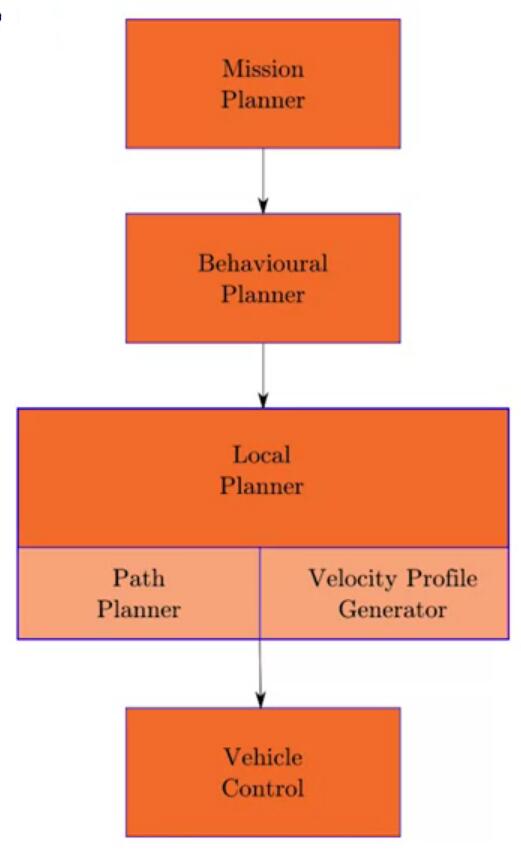
Hierarchical Motion Planning
Hierarchical Planner
- Motion planning broken into hierarchy of subproblems
- Mission planner: the highest level, focuses on map-level navigation
- Behavioural planner focuses on other agents, rules of the road, driving behaviours
- Local planner focuses on generating feasible, collision-free paths
Mission Planner
- Highest level planner
- Focuses on autonomous driving mission
- Navigate to destination at the map level
- Abstract away lower level details
- Can be solved with graph-based methods (Dijkstra’s, A*)
Behavioural Planner
- Behavioural planner decides when it is safe to proceed
- Takes pedestrians, vehicles, cyclists into consideration
- Also looks at regulatory elements, such as traffic lights and stop signs
- Finite State Machines
- Composed of states and transitions
- States are based on perception of surroundings
- Transitions are based on inputs to the driving scenario (e.g.stop lights changing colour)
- FSM is memoryless: Transitions only depend on input and current state, and not on past state sequence
- Rule-based System
- Rule-based systems use a hierarchy of rules to determine output behaviour
- Rules are evaluated based on logical predicates
- Higher priority rules have precedence
- Example scenario with two rules
- green light A intersection → drive straight
- pedestrian A driving straight → emergency stop
- Reinforcement learning
- $R = \sum^\infty_{t=0} \gamma^t R_{a_t}(s_t, s_{t+1})$
Local Planner
- Local planning generates feasible, collision-free paths and comfortable velocity profiles
- Decomposed into path planning and velocity profile generation
Path planner:
- The key ingenuity behind developing a good path planning algorithm is reducing the search space for optimization
- Three main categories of path planners: sampling-based planners, variational planners and lattice planners
- Sampling-based Planners:
- Randomly sample the control inputs to quickly explore the workspace
- One of the most iconic sampling-based algorithms is the Rapidly Exploring Random Tree or RRT
- These algorithms construct the branches of the tree of paths by generating points in randomly sampled locations and planning a path to the point, from the nearest point in the tree.
- If the path is free from collisions with any static obstacles, that path is added to the tree.
- This tree quickly explores the workspace with many potential paths and when a goal region is reached, the path that terminates in that region is returned.
- Often very fast, but can generate poor-quality paths
- Variational planners:
- rely on the calculus of variations to optimize a trajectory function which maps points in time to positions in the workspace according to some cost-functional that takes obstacles and robot dynamics into consideration. $min_{\delta x} J(x+\delta x)$
- are usually trajectory planners, which means they combine both path planning and velocity planning into a single-step.
- Can be slower, and less likely to converge to a feasible solution
- a variational method is the chomp algorithm
- Lattice Planners
- Constrain the search space by limiting actions available to the robot
- Set of actions known as control set
- This control set, when paired with a discretization of the workspace, implicitly defines a graph. This graph can then be searched using a graph search algorithm such as Dijkstra’s or A*, which results in fast computation of paths
- While the lattice planner is often quite fast, the quality of paths are sensitive to the selected control set.
- A common variance on the lattice planner is known as the conformal lattice planner, where goal points are selected some distance ahead of the car, laterally offset from one another with respect to the direction of the road and a path is optimized to each of these points.
- Conformal lattice planner fits the control actions to the road structure
- Constrain the search space by limiting actions available to the robot
Velocity profile generation:
- is usually set up as a constrained optimization problem.
- we would combine many of the velocity profile objectives such as the goals of minimizing jerk or minimizing deviation from a desired reference, the rectangle of comfortable acceleration
- Once the objectives and constraints are formalized, it becomes a matter of solving the problem efficiently. One way to do this is to calculate convex approximations to the optimization domain and objectives, which helps ensure that our optimizer doesn’t get stuck in local minima.